Measures of Central Tendency (3M)
A measure of central tendency is a single value that attempts to describe a set of data by identifying the central position within that set of data. The three most common measures are the mean, median, and mode. Here we will learn how to calculate them and under what conditions they are most appropriate to be used :
1. Mean (Arithmetic)
The mean (or average) is the most popular and well known measure of central tendency. It can be used with both discrete and continuous data, although its use is most often with continuous data (see our Types of Variable guide for data types). The mean is equal to the sum of all the values in the data set divided by the number of values in the data set. So, if we have n values in a data set and they have values x1,x2, …,xn, the sample mean, usually denoted by x̄ is:
x̄ = ( x1+x2+… + xn ) / n
This formula is usually written in a slightly different manner using the Greek capitol letter, ∑, pronounced “sigma”, which means “sum of…”:
x̄ =( ∑xn ) / n
You may have noticed that the above formula refers to the sample mean. In statistics, samples and populations have very different meanings and these differences are very important, even if, in the case of the mean, they are calculated in the same way. To acknowledge that we are calculating the population mean and not the sample mean, we use the Greek lower case letter “mu”, denoted as
μ = ( ∑xn ) / n
2. Median
The median is the middle score for a set of data that has been arranged in order of magnitude. The median is less affected by outliers and skewed data.
How to Find Median :
- Arrange the data in ascending order.
- If n (number of data points) is odd, the median is the middle value.
- If n is even, the median is the average of the two middle values.
In order to calculate the median, suppose we have the data below:
| 65 | 55 | 89 | 56 | 35 | 14 | 56 | 55 | 87 | 45 | 92 |
We first need to rearrange that data into order of magnitude (smallest first):
| 14 | 35 | 45 | 55 | 55 | 56 | 56 | 65 | 87 | 89 | 92 |
Our median mark is the middle mark – in this case, 56 (highlighted in bold).
3. Mode
The mode is the most frequent score in our data set. Normally, the mode is used for categorical data where we wish to know which is the most common category.
For Example :
i) Dataset : [2,3,3,4,5,5,5] → Mode = 5.
ii) Dataset : [2,2,3,3,4] → Modes = 2 and 3 (bimodal).
import numpy as np
from scipy import stats
import matplotlib.pyplot as plt
# Dataset
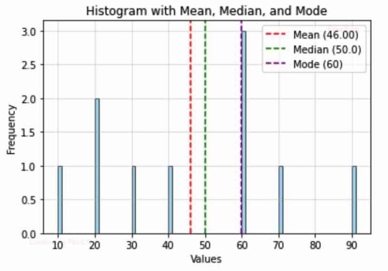
data = [10, 20, 20, 30, 40, 60, 60, 60, 70, 90]
# Calculations
mean = np.mean(data) # Mean
median = np.median(data) # Median
mode = stats.mode(data).mode[0] # Mode
# Printing the results
print(f"Mean: {mean}")
print(f"Median: {median}")
print(f"Mode: {mode}")
# Plotting the data
plt.hist(data, bins=range(min(data), max(data) + 2), color='skyblue', edgecolor='black', alpha=0.7)
plt.axvline(mean, color='red', label=f'Mean ({mean:.2f})', linestyle='dashed', linewidth=1.5)
plt.axvline(median, color='green', label=f'Median ({median})', linestyle='dashed', linewidth=1.5)
plt.axvline(mode, color='purple', label=f'Mode ({mode})', linestyle='dashed', linewidth=1.5)
# Diagram styling
plt.title('Histogram with Mean, Median, and Mode')
plt.xlabel('Values')
plt.ylabel('Frequency')
plt.legend()
plt.grid(alpha=0.4)
plt.show()