Inferential Statistics
Inferential statistics involves making predictions, decisions, or generalization about a population based on data collected from a sample. It uses probability theory to infer properties of a population, allowing us to draw conclusions that go beyond the immediate data.
Let’s go one by one all the types in Inferential Statistics :
1. Estimation
Estimation involves predicting or inferring a population parameter based on a sample statistic.
There are 2 types of Estimation
a) Point Estimation : Provides a single value as an estimate for the population parameter. For example : Using the sample mean (x̄) to estimate the population mean (μ).
b) Interval Estimation : Provides a range of values (confidence interval) within which the parameter is expected to lie. For example: A 95% confidence interval for the mean.
import numpy as np
import scipy.stats as stats

# Sample data
data = np.random.normal(loc=100, scale=15, size=50)

# Calculate mean and standard error
sample_mean = np.mean(data)
std_error = stats.sem(data)

# Confidence interval (95%)
conf_interval = stats.t.interval(0.95, len(data)-1, loc=sample_mean, scale=std_error)
print(f"95% Confidence Interval: {conf_interval}")
#Output = 95% Confidence Interval: (97.60529694628278, 106.88018606816905)
2. Hypothesis Testing
Hypothesis testing determines whether there is enough evidence in the sample data to support or reject a claim about a population parameter.
Below are the steps to check Hypothesis Testing :
- Define the null hypothesis (H0) and alternative hypothesis (Ha).
- Choose a significance level (𝛼), typically 0.05.
- Calculate the test statistic and p-value.
- Compare the p-value with α\alphaα.
- Reject or fail to reject H0.
Below are the common Hypothesis Tests :
- t-tests : Compare means between one or two groups (e.g., one-sample, independent, or paired t-tests).
- z-tests : Similar to t-tests but used when the sample size is large (n>30) and population variance is known.
- Chi-Square Tests : Used for categorical data to test relationships between variables or goodness of fit.
- ANOVA (Analysis of Variance) : Compares means across three or more groups.
# Hypothesis: Population mean is 105
t_stat, p_value = stats.ttest_1samp(data, 105)
print(f"T-statistic: {t_stat}, P-value: {p_value}")

if p_value < 0.05:
    print("Reject the null hypothesis.")
else:
    print("Fail to reject the null hypothesis.")
    # T-statistic: -1.1948214818199263, P-value: 0.2379081228478694
    # Fail to reject the null hypothesis.
3. Regression Analysis :
Regression analysis examines the relationship between dependent and independent variables.
Below are the types of Regression :
- Linear Regression : Models the relationship between two continuous variables. Example: Predicting sales based on advertising spend.
- Multiple Linear Regression : Explores relationships between one dependent variable and multiple independent variables.
- Logistic Regression : Used for binary outcomes (e.g., success/failure).
import statsmodels.api as sm

# Example data
X = np.random.normal(50, 10, 100)
y = 2 * X + np.random.normal(0, 5, 100)

# Add constant to predictor
X = sm.add_constant(X)

# Fit regression model
model = sm.OLS(y, X).fit()
print(model.summary())

#Below is the Output :
                            OLS Regression Results
==============================================================================
Dep. Variable:                      y   R-squared:                       0.958
Model:                            OLS   Adj. R-squared:                  0.958
Method:                 Least Squares   F-statistic:                     2251.
Date:                Sat, 18 Jan 2025   Prob (F-statistic):           2.04e-69
Time:                        20:51:31   Log-Likelihood:                -292.99
No. Observations:                 100   AIC:                             590.0
Df Residuals:                      98   BIC:                             595.2
Df Model:                           1
Covariance Type:            nonrobust
==============================================================================
                 coef    std err          t      P>|t|      [0.025      0.975]
------------------------------------------------------------------------------
const          2.4268      2.188      1.109      0.270      -1.915       6.769
x1             1.9579      0.041     47.447      0.000       1.876       2.040
==============================================================================
Omnibus:                        0.157   Durbin-Watson:                   1.861
Prob(Omnibus):                  0.925   Jarque-Bera (JB):                0.327
Skew:                           0.055   Prob(JB):                        0.849
Kurtosis:                       2.742   Cond. No.                         254.
==============================================================================
4. Correlation Analysis :
Measures the strength and direction of a relationship between two variables.
Below are the types of Correlation :
- Positive Correlation: Both variables increase together.
- Negative Correlation: One variable increases as the other decreases.
- No Correlation: No relationship between variables.
from scipy.stats import pearsonr

# Generate random data
x = np.random.normal(50, 10, 100)
y = 2 * x + np.random.normal(0, 5, 100)

# Calculate correlation
correlation, _ = pearsonr(x, y)
print(f"Pearson Correlation: {correlation}")
#Output = Pearson Correlation: 0.9774980072997437
5. Analysis of Variance (ANOVA) :
ANOVA compares the means of three or more groups to determine if at least one group differs significantly.
Below are the types of ANOVA :
- One-Way ANOVA : Tests the impact of a single factor on a dependent variable.
- Two-Way ANOVA : Examines the effects of two factors and their interaction.
from scipy.stats import f_oneway

# Sample data for three groups
group1 = np.random.normal(100, 10, 30)
group2 = np.random.normal(110, 15, 30)
group3 = np.random.normal(120, 20, 30)

# Perform ANOVA
f_stat, p_value = f_oneway(group1, group2, group3)
print(f"F-statistic: {f_stat}, P-value: {p_value}")
#Output = F-statistic: 15.451854630950878, P-value: 1.8098501569612255e-06
6. Non-Parametric Tests :
Used when data doesn’t meet assumptions of normality or when dealing with ordinal data.
Below are the common Non-Parametric Tests :
- Mann-Whitney U Test: Compare medians of two independent groups.
- Wilcoxon Signed-Rank Test: Compare medians of paired samples.
- Kruskal-Wallis Test: Compare medians across multiple groups.
from scipy.stats import mannwhitneyu

# Sample data for two groups
group1 = np.random.normal(100, 10, 30)
group2 = np.random.normal(110, 10, 30)

# Perform Mann-Whitney U Test
u_stat, p_value = mannwhitneyu(group1, group2)
print(f"U-statistic: {u_stat}, P-value: {p_value}")

#Output = U-statistic: 246.0, P-value: 0.0013121400321819178
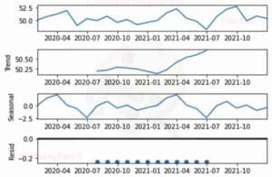
7. Time Series Analysis :
Analyzes data points collected or observed over time to identify trends, seasonal patterns, and forecast future values.
import pandas as pd
from statsmodels.tsa.seasonal import seasonal_decompose

# Simulated time series data
date_rng = pd.date_range(start='1/1/2020', end='12/31/2021', freq='M')
data = 50 + np.sin(np.linspace(0, 24, len(date_rng))) + np.random.normal(0, 1, len(date_rng))
time_series = pd.Series(data, index=date_rng)

# Decompose time series
decomposition = seasonal_decompose(time_series, model='additive')
decomposition.plot()
plt.show()
8. Chi-Square Tests :
Tests relationships between categorical variables or compares observed and expected frequencies.
Below are the types of Chi-Square Tests :
- Chi-Square Test of Independence : Examines if two categorical variables are related.
- Chi-Square Goodness-of-Fit Test : Tests if a sample matches an expected distribution.
from scipy.stats import chi2_contingency

# Contingency table
data = [[10, 20, 30],
        [15, 25, 35]]

# Perform Chi-Square Test
chi2, p, dof, expected = chi2_contingency(data)
print(f"Chi-Square Statistic: {chi2}, P-value: {p}")
# Output = Chi-Square Statistic: 0.27692307692307694, P-value: 0.870696738961232
9. Factor Analysis :
Used to identify underlying factors or dimensions within a dataset.
from sklearn.decomposition import FactorAnalysis

# Simulated dataset
data = np.random.rand(100, 5)

# Perform Factor Analysis
fa = FactorAnalysis(n_components=2)
fa.fit(data)
print(f"Factors: {fa.components_}")
# Output = Factors: [[ 0.08691678  0.11837905 -0.21500766 -0.09306249  0.00129438]
 [-0.03217917  0.14373268  0.0839336  -0.1019149  -0.07257098]]
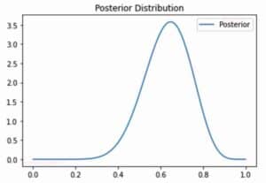
10. Bayesian Inference :
Bayesian inference incorporates prior knowledge or beliefs into statistical analysis.
from scipy.stats import beta

# Prior beliefs (Beta distribution)
alpha_prior = 2
beta_prior = 2

# Observed data (successes and failures)
successes = 10
failures = 5

# Posterior distribution
alpha_post = alpha_prior + successes
beta_post = beta_prior + failures

# Visualize posterior
x = np.linspace(0, 1, 100)
posterior = beta.pdf(x, alpha_post, beta_post)

import matplotlib.pyplot as plt
plt.plot(x, posterior, label='Posterior')
plt.title("Posterior Distribution")
plt.legend()
plt.show()